[18]:
suppressMessages(library(Seurat))
suppressMessages(library(dplyr))
suppressMessages(library(tidyverse))
suppressMessages(library(viridis))
suppressMessages(library(ggalluvial))
suppressMessages(library("ggsci"))
suppressMessages(library("ggplot2"))
suppressMessages(library("gridExtra"))
library(cowplot)
APCside gene expression#
[3]:
my24_1colors <- c('#53868B','#00F5FF','#7FFFD4','#C1FFC1','#0000FF','#7B68EE',
                  '#CDCD00','#FFF68F','#CD9B1D','#8B658B','#FF6A6A','#8B3A3A',
                  '#1E90FF','#FF69B4','#8DB6CD','#CAE1FF','#EECFA1','#8B7B8B',
                  '#4F4F4F','#FF4500','#BC8F8F','#FFA500','#228B22','#8B4513')

my23colors <- c('#53868B','#00F5FF','#C1FFC1','#0000FF','#7B68EE',
                  '#CDCD00','#FFF68F','#CD9B1D','#8B658B','#FF6A6A','#8B3A3A',
                  '#1E90FF','#FF69B4','#8DB6CD','#CAE1FF','#EECFA1','#8B7B8B',
                  '#4F4F4F','#FF4500','#BC8F8F','#FFA500','#228B22','#8B4513')
[86]:
modify_vlnplot<- function(obj,
features,
pt.size = 0,
plot.margin = unit(c(-0.75, 0, -0.75, 0), "cm"),
cols=my23colors,
slot="data",
assay="RNA",
...) {
p <- VlnPlot(obj, features = features, pt.size = pt.size, cols=cols, slot=slot,
assay=assay,... ) + theme_bw() +
xlab("") + ylab(features) + ggtitle("") +
theme(legend.position = "none",
panel.grid=element_blank(),
axis.text.x = element_blank(),
axis.text.y = element_blank(),
#axis.ticks.x = element_blank(),
#axis.ticks.x = element_line(color="red"),
axis.ticks.length = unit(0, "pt"),
#axis.ticks.y = element_line(color="red"),
axis.ticks.y = element_blank(),
plot.title= element_blank(),
axis.title.x = element_blank(),
#axis.title.x = element_text(size = rel(1), angle = 45, vjust = 0),
axis.title.y = element_text(size = rel(1), angle=0, vjust = 0.5, hjust = 0),
plot.margin = plot.margin, axis.line.x=element_blank())
#plot.margin = plot.margin) +
#annotate(
# geom = 'segment',
# y = -Inf,
# yend = Inf,
# x = Inf,
# xend = Inf
# )
return(p)
}
## main function
StackedVlnPlot<- function(obj, features,
pt.size = 0,
slot="data",
assay="RNA",
plot.margin = unit(c(-0.75, 0, -0.75, 0), "cm"),
...) {
plot_list<- purrr::map(features, function(x) modify_vlnplot(obj = obj, features = x, slot=slot, assay=assay,...))
plot_list[[1]] <- plot_list[[1]] + theme(legend.position = "top", axis.line.x=element_blank())
#plot_list[[1]] <- plot_list[[1]] + theme(panel.background = element_rect(fill = 'grey75'))
#plot_list[[1]] <- plot_list[[1]] + scale_x_continuous(position="top")
#plot_list[[1]] <- plot_list[[1]] + annotate(geom = 'segment', y = Inf, yend = Inf, x = -Inf, xend = Inf, size=0.5 )
plot_list[[length(plot_list)]]<- plot_list[[length(plot_list)]] +
theme(axis.text.x=element_text(size = rel(1), angle = 45, vjust = 1, hjust = 1),
axis.ticks.x = element_line(), axis.ticks.length = unit(5, "pt"))
#axis.line.x=element_line(linetype=1,color="black",size=0.5))
#+
#theme(axis.title.y=element_text(size = rel(1), angle = 0, vjust = 0.5, hjust = 0), axis.ticks.y = element_blank())
#plot_list[[1]]
#print(names(plot_list))
#p <- do.call(what = '+', args = plot_list)
#p <- p + theme_cowplot()
#p <- p + scale_x_continuous(
# expand = c(0, 0),
# labels = function(x) c(rep(x = '', times = length(x)-2), x[length(x) - 1], '')
# )
#
#p <- patchwork::wrap_plots(plotlist = plot_list, ncol = 1 )
#+ theme(plot.margin = plot.margin))
#p <- p + theme(plot.margin = plot.margin)
p <- plot_list[[1]]
for (i in 2:length(plot_list)){
p <- p + plot_list[[i]]
}
return(p)
}
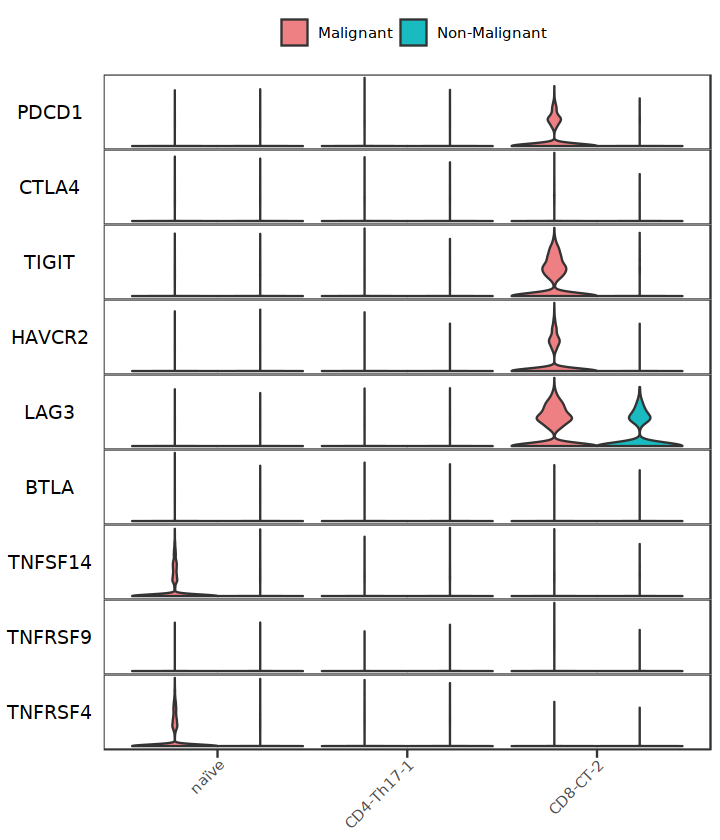
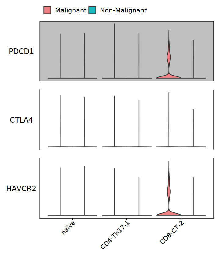
StackedVlnPlot(subT, features=Tside_genes2, split.by="status2", cols= c('#EE8084','#19BBC1'))
#theme(plot.margin = unit(c(-0.75, 0, -0.75, 0), "cm")) + theme_cowplot() +
#theme(panel.spacing.x = unit(10, "cm"),
# panel.spacing.y = unit(-1, "cm")
# )
#ggsave("aaaaaa.pdf", w=8, h=7)
[ ]:
[8]:
Tside_genes2 <- c("PDCD1", "CTLA4", "HAVCR2")
subT <- subset(Tcell, cell.type.sub %in% c("CD4-Th17-1", "naïve", "CD8-CT-2"))
data <- as.data.frame(
    x = as.matrix(
        x = t(as.matrix(x = GetAssayData(
            object = subT,
            slot = "data")[Tside_genes2, rownames(subT@meta.data), drop = FALSE]))))


Melt <- function(x) {
  if (!is.data.frame(x = x)) {
    x <- as.data.frame(x = x)
  }
  return(data.frame(
    rows = rep.int(x = rownames(x = x), times = ncol(x = x)),
    cols = unlist(x = lapply(X = colnames(x = x), FUN = rep.int, times = nrow(x = x))),
    vals = unlist(x = x, use.names = FALSE)
  ))
}

data <- Melt(data)

idents <- subT[["cell.type.sub", drop = TRUE]]


data2 <- data.frame(
    feature = data$cols,
    expression = data$vals,
    ident = rep_len(x = idents, length.out = nrow(x = data))
  )

geom <- list(geom_violin(scale = 'width', adjust = 1, trim = TRUE))

plot <- ggplot(
    data = data2,
    mapping = aes_string(x = "ident", y="expression", color = "feature", fill="feature")
  ) +
    #labs(x = xlab, y = ylab, title = feature, fill = NULL) +
    theme_cowplot() +
    theme(plot.title = element_text(hjust = 0.5))

#plot <- do.call(what = '+', args = list(plot, geom))

plot + geom

plot
Error in subset(Tcell, cell.type.sub %in% c("CD4-Th17-1", "naïve", "CD8-CT-2")): 找不到对象'Tcell'
Traceback:

1. subset(Tcell, cell.type.sub %in% c("CD4-Th17-1", "naïve", "CD8-CT-2"))
[ ]:
[9]:
setwd("/annoroad/data1/bioinfo/PROJECT/big_Commercial/Cooperation/B_TET/B_TET-003/std/result/fanxuning/commander_test/THU/")
[10]:
Mye_final <- readRDS("final_Mye_20220805.RDS")
[11]:
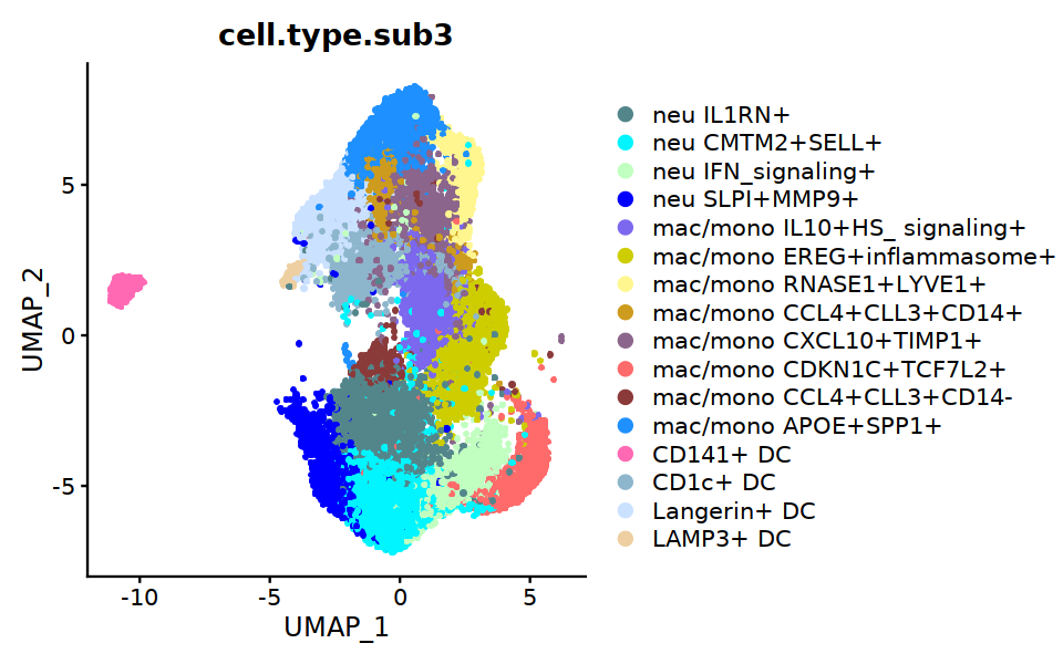
options(repr.plot.width=8, repr.plot.height=5)

DimPlot(Mye_final,  group.by="cell.type.sub3", raster=TRUE, cols=my23colors,
        label=FALSE,pt.size=3)
[12]:
unique(Mye_final@meta.data$cell.type.sub3)
- CD141+ DC
- mac/mono IL10+HS_ signaling+
- neu SLPI+MMP9+
- CD1c+ DC
- Langerin+ DC
- mac/mono EREG+inflammasome+
- mac/mono RNASE1+LYVE1+
- neu IFN_signaling+
- mac/mono CCL4+CLL3+CD14+
- mac/mono CXCL10+TIMP1+
- mac/mono CDKN1C+TCF7L2+
- neu IL1RN+
- neu CMTM2+SELL+
- mac/mono CCL4+CLL3+CD14-
- mac/mono APOE+SPP1+
- LAMP3+ DC
Levels:
- 'neu IL1RN+'
- 'neu CMTM2+SELL+'
- 'neu IFN_signaling+'
- 'neu SLPI+MMP9+'
- 'mac/mono IL10+HS_ signaling+'
- 'mac/mono EREG+inflammasome+'
- 'mac/mono RNASE1+LYVE1+'
- 'mac/mono CCL4+CLL3+CD14+'
- 'mac/mono CXCL10+TIMP1+'
- 'mac/mono CDKN1C+TCF7L2+'
- 'mac/mono CCL4+CLL3+CD14-'
- 'mac/mono APOE+SPP1+'
- 'CD141+ DC'
- 'CD1c+ DC'
- 'Langerin+ DC'
- 'LAMP3+ DC'
[13]:
mye_cs <- c("CD141+ DC", "CD1c+ DC", "LAMP3+ DC", "Langerin+ DC", "")
[14]:
Tcell <- readRDS("T_clean_5thAnnotation.rds")

Tcell@meta.data$status2 <- "Malignant"
Tcell@meta.data[Tcell@meta.data$status == "P", "status2"] <- "Non-Malignant"
Tcell@meta.data[Tcell@meta.data$status == "T", "status2"] <- "Malignant"

Tcell@meta.data$status2 <- factor(Tcell@meta.data$status2,levels = c("Malignant", "Non-Malignant"))
#
Tcell@meta.data$treat <- "NoTreat"
Tcell@meta.data[Tcell@meta.data$patient == "MIBC5", "treat"] <- "Treat"
Tcell@meta.data[Tcell@meta.data$patient == "MIBC6", "treat"] <- "Treat"
Tcell@meta.data[Tcell@meta.data$patient == "MIBC8", "treat"] <- "Treat"
Tcell@meta.data[Tcell@meta.data$patient == "MIBC13", "treat"] <- "Treat"

Tcell@meta.data$status_treat <- paste(Tcell@meta.data$status2, Tcell@meta.data$treat, sep="_")
[15]:
Tcell@meta.data$treat <- factor(Tcell@meta.data$treat, levels=c("Treat", "NoTreat"))
[16]:
Idents(Tcell) <- "cell.type.sub"
[87]:
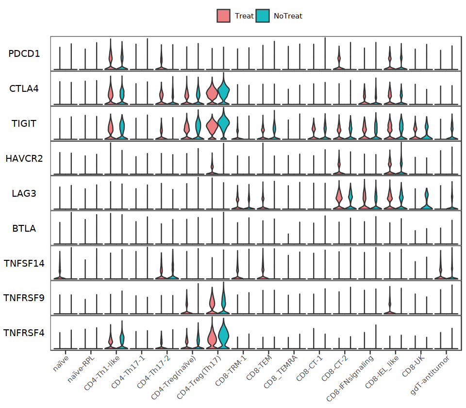
options(repr.plot.width=8, repr.plot.height=7)

Tside_genes2 <- c("PDCD1", "CTLA4", "TIGIT", "HAVCR2", "LAG3", "BTLA", "TNFSF14", "TNFRSF9", "TNFRSF4")
#Tside_genes2 <- c("PDCD1", "CTLA4")
StackedVlnPlot(Tcell, features=Tside_genes2, split.by="treat", cols= c('#EE8084','#19BBC1'), pt.size = 0) + theme(legend.position = "right")
ggsave("20220810_Tside_genes.pdf", w=8, h=7)
[ ]:
[26]:
Tside_genes2 <- c("PDCD1", "CTLA4", "HAVCR2")
subT <- subset(Tcell, cell.type.sub %in% c("CD4-Th17-1", "naïve", "CD8-CT-2"))
[48]:
StackedVlnPlot(subT, features=Tside_genes2, split.by="status2", cols= c('#EE8084','#19BBC1')) +
    #theme(plot.margin = unit(c(-0.75, 0, -0.75, 0), "cm")) + theme_cowplot() +
    theme(panel.spacing.x = unit(10, "cm"),
          panel.spacing.y = unit(-1, "cm")
         )
[ ]:
[ ]:
[ ]:
DC macrophage#
[20]:
APC <- readRDS("/annoroad/data1/bioinfo/PROJECT/big_Commercial/Cooperation/B_TET/B_TET-072/supplement/yaojiaying/AN202202140002/Analysis/Data/Fig5_APC.rds")
[21]:
APC$cluster<-factor(APC$cluster,levels=c('CD141+ DC','CD1c+ DC','LAMP3+ DC','Langerin+ DC','pDC','Neutrophil','Macrophage','Monocyte','MonoDC','MCt','MCtc'))

tmp1<-subset(APC,cluster %in% c('Macrophage','Monocyte','MonoDC')) #合并后Mac 3个群
tmp2<-subset(APC,cluster %in% c('MCt','MCtc')) #合并后Mast 2个群

tmp1$cluster<-as.vector(tmp1$cluster)
tmp2$cluster<-as.vector(tmp2$cluster)
[22]:
subAPC <- subset(APC, cluster != "pDC")
[23]:
subAPC@meta.data$treat <- "NoTreat"
subAPC@meta.data[subAPC@meta.data$patient == "MIBC5", "treat"] <- "Treat"
subAPC@meta.data[subAPC@meta.data$patient == "MIBC6", "treat"] <- "Treat"
subAPC@meta.data[subAPC@meta.data$patient == "MIBC8", "treat"] <- "Treat"
subAPC@meta.data[subAPC@meta.data$patient == "MIBC13", "treat"] <- "Treat"
[24]:
subAPC@meta.data$treat <- factor(subAPC@meta.data$treat, levels=c("Treat", "NoTreat"))
[88]:
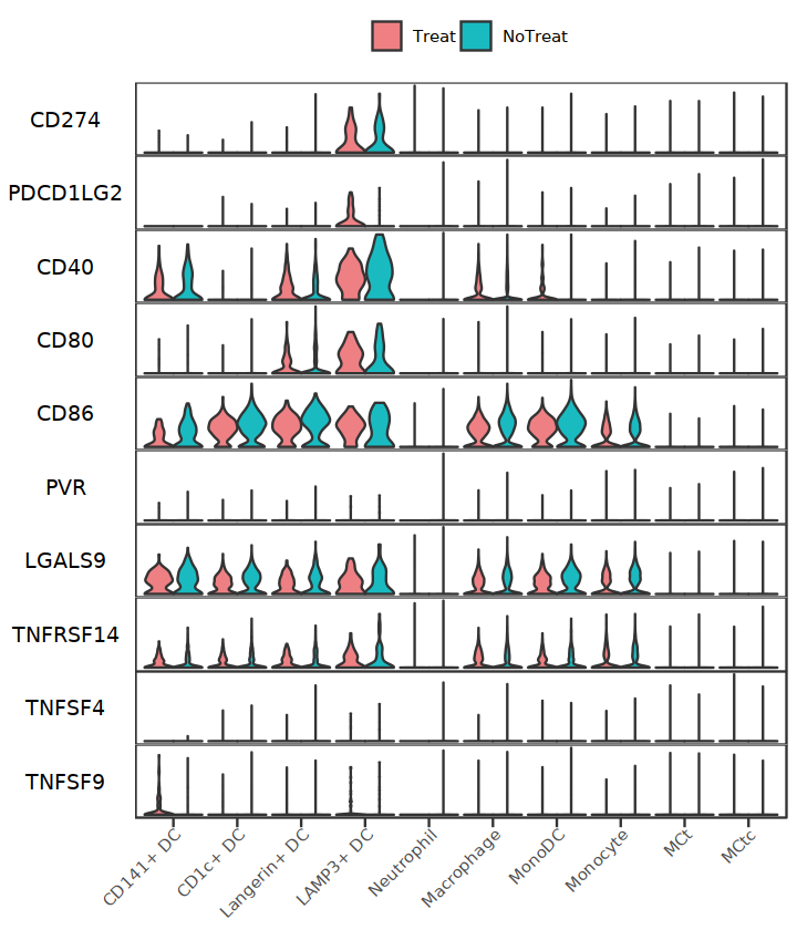
APC_side_genes <- c("CD274","PDCD1LG2","CD40","CD80","CD86","PVR","LGALS9","TNFRSF14","TNFSF4","TNFSF9")
options(repr.plot.width=6, repr.plot.height=7)
StackedVlnPlot(subAPC, features=APC_side_genes, split.by="treat", cols= c('#EE8084','#19BBC1'), pt.size = 0)
ggsave("20220810_APCside_genes.pdf", w=6, h=7)
[ ]:
[ ]:
[ ]:
[ ]:
[ ]: